In this chapter we show that many types of questions about data in a database can be interpreted and answered geometrically.
If each entry in a database contains $d$ different data, we can interpret these data as coordinates in the space $\mathbb R^d$, and we can imagine the database as a set of points in $\mathbb R^d$.
Often, we can meet a task to find those items in the database whose individual data are within a specified range. This leads to the geometric task of orthogonal searching.
Formulation of a general orthogonal search task in $\mathbb R^d$
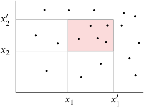
In $\mathbb R^d$ there is a set of points $P$. The task of orthogonal range searching consists in finding a suitable search structure made just for this set which enables us to find quickly all points from $P$ lying inside a $d$-dimensional axis-parallel box
for any choice of intervals $[x_1,x_1']$, $[x_2,x_2']$, $\dots$, $[x_d,x_d']$.
Figure 7.1 The task of orthogonal range searching
We will deal with two ways how to solve this task. The appropriate search structures are called kd-trees and range trees.
We start with dimension $1$ in which both methods coincide.
$1$-dimensional range searching
Let $P=\{p_1,p_2,\dots, p_n\}$ be a set of real numbers. To order them according
to the size we can construct a balanced binary tree $\mathcal T$ with
leaves corresponding to these numbers. For given numbers $x$ and $x'$, $x\leq x'$, we look for all the numbers of the set $P$ that lie in the interval $[x, x ']$. In the tree $\mathcal T$, each node will hold the value of the largest leaf of its left subtree. Then in the tree every number $x$ determines a path from the root to a leaf that is specified by the rule that from a given node we go left if $x$ is less than or equal to the value at that node, and we go right in the opposite case.
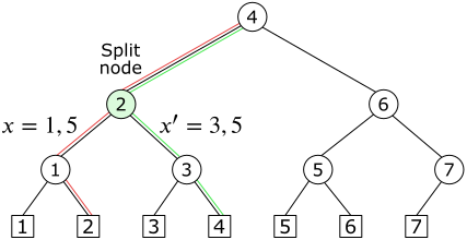
The given numbers $x$ and $x'$ specify two paths that have a common part. The last node of this common part is called a split node.
Figure 7.2 A split node for $x=1,5$ and $x'=3,5$. The path of $x$ is marked in red, the path of $x'$ in green.
For a node $\nu$ of the tree $\mathcal T$ let $\operatorname{lc}(\nu)$ and $\operatorname{rc}(\nu)$ denote its left and right child, respectively. A pseudocode for finding a split node is as follows:
FindSplitNode$(\mathcal T, x, x')$
Input. A tree $\mathcal T$ and two values $x$ and $x'$ with $x\leqslant x'$.
Output. The node $v$ where the paths to $x$ and $x'$ split, or the leaf where both paths end.
$v\leftarrow root(\mathcal T)$
while $v$ is not a leaf and $(x'\leqslant x_v$ or $x\gt x_v)$
do if $x'\leqslant x_v$
then $v\leftarrow lc(v)$
else $v\leftarrow rc(v)$
return $v$
The pseudocode for finding the points from the set $P$ located in the interval $[x, x']$ finds the split node first, and then continues to look for the position of the numbers
$x$ and $x'$ among the leaves of the tree $\mathcal T$.
then Check if the point stored at $v_{\text{split}}$ must be reported.
else (* Follow the path to $x$ and report the points in subtrees right of the path. *)
$v\leftarrow lc(v_{\text{split}})$
while $v$ is not a leaf
do if $x\leqslant x_v$
thenReportSubtree(rc($v$))
$v\leftarrow lc(v)$
else $v\leftarrow rc(v)$
Check if the point stored at the leaf $v$ must be reported.
Similarly, follow the path to $x'$, report the points in subtrees left of the path, and check if the point stored at the leaf where the path ends must be reported.
Denote $k$ the number of elements of the set $P$ that are in the interval $[x,x']$. Then the time needed to be listed is $O(\log n+k)$.
kd-trees in dimension 2
Now let $P=\{p_1,p_2,\dots, p_n\}$ be a set of points in the plane $\mathbb R^2$.
To simplify and clarify geometric interpretation we assume that there are no points in $P$ that have the same either $x$ or $y$-coordinate. In time, we will show how to remove this limiting assumption.
The kd-tree for the set $P$ will have the geometric form of a division of the plane into regions by means of vertical and horizontal lines, half-lines and segments. The division is made in such a way that each region contains just one point of the set $P$. We describe this geometric division using a balanced binary tree called a kd-tree.
First we find a point of the set $P$ with the property that the vertical line $l_1$ passing this point divides the set $P$ into two parts $P_1$ and $P_2$ such that the number of elements of the left part $P_1$ is the same or bigger by one than the number of elements of the right part $P_2$. In the set $P_2$ we include the points to the right of the line $l_1$, the other points are in the set $P_1$. This means that the $x$-coordinate of a point through which the vertical line $l_1$ goes will be the median of the $x$-coordinates of the points of $P$. In the kd-tree this geometric step corresponds with the selection of a root in which we will hold the vertical line $ l_1 $ together with its $x$-coordinate. The path from the root to left means a passage to the set $P_1$, the path to right a passage to $P_2$.
In the next step, we analogously divide both sets of $ P_1 $ and $ P_2 $ with the horizontal lines $l_2$ and $l_3$ to two sets. The lower one contains a point on the splitting horizontal half-line and it has the same number of points or one point more than the upper set. In the kd-tree, lines $l_2$ and $l_3$ will match the left and right child of the node $l_1$, respectively.
The obtained sets -- now they are four -- are again divided alternately by vertical and horizontal lines into sets whose numbers of elements differ by no more than one. We repeat this procedure until there is only one point in the obtained sets. The whole procedure is captured in the following animation.
After finishing we get a balanced binary tree, where the nodes on even levels store the $x$-coordinate of the corresponding vertical line, and the nodes on odd levels
store the $y$-coordinate of the corresponding horizontal line.
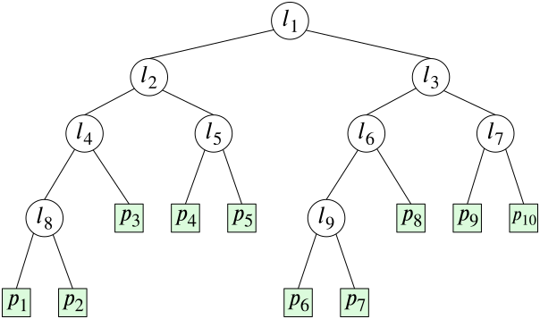
Figure 7.3 kd-tree for the set $P$ from the animation.
kd-tree can be constructed using the recursive procedure described by the following pseudocode:
AlgorithmBuildKdTree$(P, depth)$
Input. A set of points $P$ and the current depth $depth$.
Output. The root of a kd-tree storing $P$.
if $P$ contains only one point
then return a leaf storing this point
else if $depth$ is even
then Split $P$ into two subsets with a vertical line $\ell$ through the median $x$-coordinate of the points in $P$. Let $P_1$ be the set of points to the left of $\ell$ or on $\ell$, and let $P_2$ be the set of points to the right of $\ell$.
else Split $P$ into two subsets with a horizontal line $\ell$ through the median $y$-coordinate of the points in $P$. Let $P_1$ be the set of points below $\ell$ or on $\ell$, and let $P_2$ be the set of points above $\ell$.
Create a node $v$ storing $\ell$, make $v_{\text{left}}$ the child of $v$, and make $v_{\text{right}}$ the right child of $v$.
return $v$
Lemma 7.1
kd-tree for a set of $n$ points in the plane uses $O(n)$ storage and can be constructed in $O(n\log n)$ time.
Proof
Every node and leaf in a binary tree uses $O(1)$ storage and this means that the total amount of storage is $O(n)$. The median of $n$ numbers can be found in $O(n)$ time. However, such algorithms are rather complicated. Therefore, it is better to order the points of the set $P$ according to the $x$ and $y$-coordinates first, which will take the time $ O(n\log n)$. Then finding a median of a subset will be linear in the number of elements of that subset. Denote $T(n)$ the running time of the algorithm for $n$ points on the input. We get a recurrent formula
$$T(1)=O(1),\quad T(n)=O(n)+2T(n),$$
which has the solution $T(n)=O(n\log n)$.
\(\Box\)
Searching using kd-tree
To describe a searching in kd-tree, we need the notion of the region of a node $\nu$.
Let the path from the root to a node $\nu$ in a kd-tree be formed by nodes $\nu_1$, $\nu_2$, $\dots$, $\nu_k$, $\nu$. Let a node $\nu_i$ be determined by a line $l_i$. Then the region of the node $\nu$ is the intersection of corresponding half-planes determined by the boundary lines $l_1$, $l_2$ to $l_k$.
Which of the two half-planes corresponding to a line we take is given by the path to $\nu$. If the path from a node on the even level goes left, we take the closed left half-plane, if it goes right we choose the open right half-plane. If the path from an odd level node goes left we take the closed lower half-plane, in the opposite case we choose the open upper half-plane.
Figure 7.4 The region of the node $\nu$.
If a node $\nu$ is determined by a line $l$, then the definition of the region can be recurrently described in this way:
where the line $l$ divides the plane into the closed left and (or lower) half-plane $\operatorname{left(l)}$ and the open right (or upper) half-plane $\operatorname{right(l)}$.
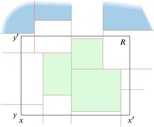
Given a rectangle $R=[x,x']\times [y,y']$ in the plane, we want to find all points from $P$, which lie in it. For the region of a node there are the following options:
The whole region lies in $R$. Then all points from this region lie in $R$.
The intersection of the region with the rectangle $R$ is empty. Then there is no point from the region in $R$.
The region has nonempty intersection with $R$, but it is not its subset. In this case we have to deal with regions corresponding to the left child and the right child of our node.
The following picture captures regions of all three types.
Figure 7.5 Regions of type (1) are green, of type (2) blue and of type (3) white.
The principle described above is realized in the following pseudocode:
AlgorithmSearchKdTree$(v, R)$
Input. The root of (a subtree of) a kd-tree, and a range $R$.
Output. All points at leaves below $v$ that lie in the range.
if $v$ is a leaf
then Report the point stored at $v$ if it lies in $R$.
else if $region(lc(v))$ is fully contained in $R$
thenReportSubtree$(lc(v))$
else if $region(lc(v))$ intersects $R$
thenSearchKdTree$(lc(v), R)$
if $region(rc(v))$ is fully contained in $R$
thenReportSubtree$(rc(v))$
else if $region(rc(v))$ intersects $R$
thenSearchKdTree$(rc(v), R)$
Without proof, we will state the following statement about the running time of searching algorithm using kd-tree.
Lemma 7.2
Let a set $P$ in the plane have $n$ points and let $k$ of them lie
in a rectangle $R$. Then the searching algorithm using kd-tree has the running time
$$O(\sqrt{n}+k).$$
So far we have done everything provided that any two points of the set $P$ have
both coordinates $x$ and $y$ different. Now we will show how this unpleasant assumption can be removed. Instead of numbers, we will consider the pairs of numbers ordered lexicographically. If a point has coordinates $(x, y)$, then its "new" coordinates are defined as pairs
$$\{(x,y),(y,x)\}.$$
Then every two different points in the plane have also both coordinates different.
We replace a rectangle $R=[x,x']\times [y,y']$ by the following rectangle in new coordinates
Therefore, we can use the above algorithms, replacing the classical coordinates with the new coordinates and using the standard lexicographical arrangement instead of
common arrangement of real numbers.
Range trees
Now we describe the second searching structure, again under the simplification assumption that no two points in the set $P$ have the same $x$ or $y$-coordinate.
The searching structure for $P$ consists of the binary tree $\mathcal T$ which has
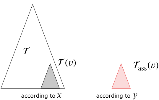
the points of the set $P$ as its leaves arranged according to the $x$-coordinate. Each node $\nu$ in $\mathcal T$ determines a subtree $\mathcal T(\nu)$ whose root it is. For each such subtree, we create an associated subtree $\mathcal T_{\rm ass}(\nu)$ which has the same points in its leaves as $\mathcal T(\nu)$ but arranged according to the coordinate $y$.
Figure 7.6 Associated subtree.
The tree $\mathcal T$ together with the system of associated subtrees
$\mathcal T_{\rm ass}(\nu)$ for all nodes $\nu$ of $\mathcal T$ is called
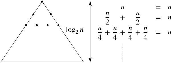
a range tree. If the set $P$ contains $n$ points, so an associated subtree
for a node $\nu$, to which we get from the root of the tree $\mathcal T$ after $i$ steps, requires storage proportional to the number of leaves, i.~e.
$$O\left(\frac{n}{2^i}\right).$$
There are $2^i$ such nodes in the tree $\mathcal T$ that is why the overall storage needed for their associated subtrees is $O(n)$. Since $i$ takes values $0,1,2,\dots,\log_2n-1$, any range tree on a set with $n$ points requires storage
$$O(n\log n).$$
This is more than the corresponding kd-tree on the same set. However searching with range trees will be faster than searching with kd-trees.
Figure 7.7 Storage requirement of a range tree on $n$ points.
A construction of a range tree is described by the following pseudocode:
AlgorithmBuild2DRangeTree$(P)$
Input. A set $P$ of points in the plane.
Output. The root of a 2-dimensional range tree.
Construct the associated structure: Build a binary search tree $\mathcal{T}_{\text{assoc}}$ on the set $P_y$ of $y$-coordinates of the points in $P$. Store at the leaves of $\mathcal{T}_{\text{assoc}}$ not just the $y$-coordinate of the points in $P_y$, but the points themselves.
if $P$ contains only one point
then Create a leaf $v$ storing this point, and make $\mathcal{T}_{\text{assoc}}$ the associated structure of $v$.
else Split $P$ into two subsets; one subset $P_{\text{left}}$ contains the points with $x$-coordinate less than or equal to $x_{\text{mid}}$, the median $x$-coordinate, and the other subset $P_{\text{right}}$ contains the points with $x$-coordinate larger than $x_{\text{mid}}$.
Create a node $v$ storing $x_{\text{mid}}$, make $v_{\text{left}}$ the left child of $v$, make $v_{\text{right}}$ the right child of $v$, and make $\mathcal{T}_{\text{assoc}}$ the associated structure of $v$.
return $v$
Orthogonal searching using range-trees.
It is based on one-dimensional searching, first according to the coordinate $x$, then according to the coordinate $y$. Let us enter intervals $[x, x ']$ and $[y, y']$. Let's begin with the search in the tree $\mathcal T$ according to the $x$-coordinate. For the interval $[x, x ']$ we find a split node. Behind it, the paths for $x$ and $x'$ diverge.
If the path for $x$ leads from a node $\nu$ to the left, then the $x$-coordinates of all the leaves of the right child $\operatorname{rc}(\nu)$ lie within the interval $[x, x ']$.
We just need to find out which of the $y$-coordinates are in the interval $[y,y']$.
We do this with one-dimensional searching in the tree $\mathcal T_{\rm ass}(\operatorname{rc}(\nu))$
With the path for $x'$ from the split node we proceed analogously. If the path from a node $\nu$ goes right, $x$-coordinates of all leaves from the left subtree of $\nu$ lie in the interval $[x,x']$ and that is why we search in the subtree
$\mathcal T _{\rm ass}(\operatorname{lc}(\nu))$ for the leaves with
$y$-coordinate in $[y,y']$. The searching algorithm is described by the following pseudocode:
Check if the point stored at $v$ must be reported.
Similarly, follow the path from $rc(v_{\text{split}})$ to $x'$, call 1DRangeQuery with the range $\left[y:y'\right]$ on the associated structures of subtrees left of the path, and check if the point stored at the leaf where the path ends must be reported.
We now show that the running time of searching with range trees is more favourable than the running time of searching with kd-trees.
Lemma 7.3
Let a set $P$ in the plane have $n$ points and let $k$ of them lie in a rectangle $R$. Then finding these points using a corresponding range tree takes time
$$O(\log^2n+k).$$
Proof
Searching in the associated subtree of the left or right child of a node $\nu$ with $n_\nu$ leaves from which $k_\nu$ leaves lie in the rectangle $R$ takes time
$$O(\log n_\nu+k_\nu).$$
So the overall time needed to find all the points of the set $P$ lying in $R$ is
$$O\left(\sum (\log n_\nu+k_\nu)\right),$$
where the sum is taken over all nodes through which the paths for $x$ and $x'$ go.
Both paths have the same length equal to the height $\log n$ of the tree.
That is why we can carry out the estimate
Both methods can be used in dimensions higher than $2$.
In the case of kd-tree in $\mathbb R^d$ we replace vertical and horizontal lines
by hyperplanes of dimension $d-1$ which are perpendicular to a coordinate axis, so there is $d$ types of these hyperplanes.
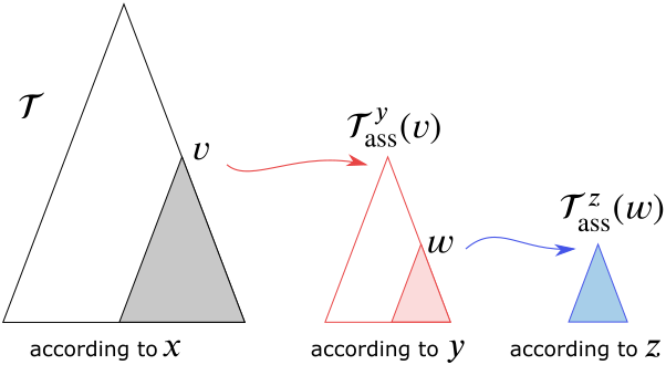
A range trees in dimension $d$ is a chain of associated subtrees. In dimension $3$ we take first the tree $\mathcal T$ giving arrangement of points in $P$ according to the coordinate $x$. To every node $\nu$ of this tree we assign an associated subtree $\mathcal T^y_{ass}(\nu)$ which determines the arrangement according to the coordinate $y$, and finally for each node $\omega$ from $\mathcal T^y_{ass}(\nu)$ we construct an associated tree $\mathcal T^z_{ass}(\omega)$ describing the arrangement according to the coordinate $z$. See Figure 7.8.
Figure 7.8 Associated subtrees in dimension 3.
Parameters of both algorithms in dimension $d\ge 2$ are described by the following table: