Point location
Introduction
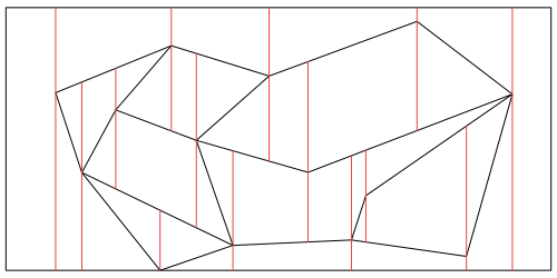
For a given planar subdivision (map), we want to find a search structure that finds in which face (region) a point lies when entering the point coordinates. The idea of the algorithm is to "refine" the subdivision into a so-called trapezoidal map, and to construct the search structure for this subdivision. The advantage of the trapezoidal map is that its individual areas are trapezoids and triangles (which can be considered as deformed trapezoids), and these can be relatively simply described using only four data.

Figure 8.1
Creation of a trapezoidal map.
Trapezoidal map
Let us have a planar subdivision (usually given by a double-connected edge list) bounded by a rectangle $ R $. This subdivision with its edges determines a set of segments that do not intersect at the inner points, but may have common end points. We construct the trapezoidal map for any such set of segments $S=\{s_1, s_2, \dots.s_n\}$ inside a rectangle $R$. To make things geometrically easier we assume that no two end points of these segments have the same $x$-coordinate. We will remove this limiting assumption later. The left end of the segment $s_i$ will be $p_i$, the right end point $q_i$.
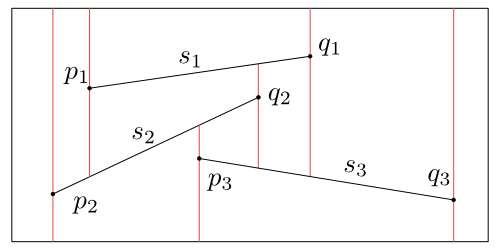
We build the trapezoidal map $\mathcal T(S)$ so that through each end point of a segment from $S$ we lead a vertical segment connecting the nearest upper segment with the nearest lower segment, see Figure 8.2. This divides the entire rectangle $R$ into trapezoids and triangles.

Figure 8.2
A trapezoidal map for three segments.
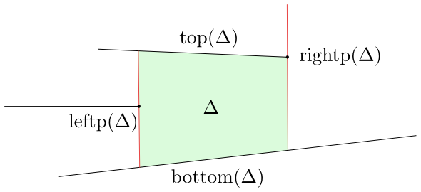
Let us show how the trapezoids and triangles of this map can be described using segments from $S$ and their end points. Each trapezoid or triangle $\Delta$ has two non-vertical sides, each being a part of a segment from $S$ or a part of the upper or lower side of the
rectangle $R$. The upper side of this trapezoid will be called $\top(\Delta)$, the lower one will be denoted as $\bo(\Delta)$. The vertical sides are determined by end points $p_j$ and $q_j$ of segments from $S$. In the case of a triangle, one of the vertical sides
reduces to a point. Therefore, every trapezoid or triangle $\Delta$ is determined by a top and a bottom and by a point $\lp(\Delta)$ through which the left vertical side passes and by a point $\rp(\Delta)$ through which the right vertical side passes.

Figure 8.3
Description of the trapezoid $\Delta$.
The substantial is that in the trapezoidal map for $n$ segments the number of vertices and trapezoids is linear in $n$.
Theorem 8.1
The trapezoidal map for $n$ segments has at most $6n+4$ vertices and $3n+1$ trapezoids.
Proof
The overall number of vertices is given by the vertices of the rectangle $R$ -- they are 4, by end points of segments -- they are at most $2n$ and by new vertices, which were made by at most $2n$ vertical segments -- they are twice the number of verticals (vertical edges), so at most $4n$.
Altogether we get at most $6n+4$ points.
We find the number of trapezoids by specifying for each point the maximum number of trapezoids $\Delta$ for which this point is the left point $\lp(\Delta)$. There is just one such trapezoid for the left lower corner of the rectangle $R$. There is one such trapezoid
for a right end point $q_i$, there are two such trapezoids for a left end point $p_i$.

Figure 8.4
Numbers of trapezoids for different kinds of left points.
Taking into account that some of end points coincide (in this case some trapezoids are counted twice), the number of all trapezoids will be at most
$$1+n+2n=3n+1.$$
\(\Box\)
Search structure
We are given a point $r$ which does not lie on any segment of $S$ and the $x$-coordinate of which differs from all $x$-coordinates of the end points $p_i$ and $q_i$. The search structure for a trapezoidal map $\mathcal T(S)$ is used to determine the trapezoid in which the specified point $r$ is located.
It is an oriented graph $\mathcal D(S)$ with the following properties:
- In leaves of the graph there are all trapezoids of the trapezoidal map $\mathcal T(S)$.
- Two edges come from every inner node.
- Inner nodes are of two following types:
- The nodes of the first type are connected with end points $p_i$ and $q_i$. From such a node (denote it for a moment as $p$) we go left if for $x$-coordinates
$r_x\lt p_x$, and we go right if $r_x\gt p_x$.
- The nodes of the second type are described by segments $s_i$. From such a node we proceed left if the point $r$ lies under the segment $s_i$, and we go right if $r$ lies over $s_i$.
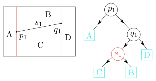
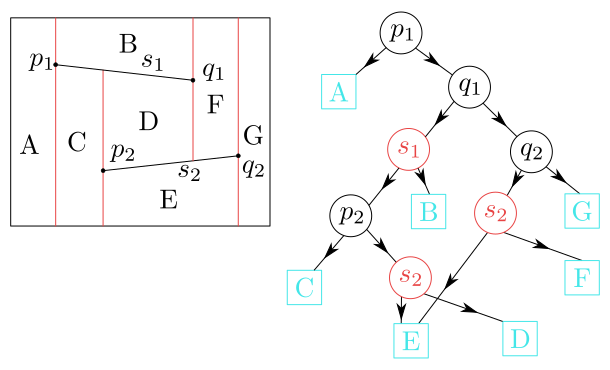
While for the specified set $S$ the trapezoid map is uniquely identified, the search structure with the above properties is not uniquely determined. The following figures give simple examples of trapezoidal maps and related search structures.

Figure 8.5
Trapezoidal map and a search structure for 1 segment.

Figure 8.6
Trapezoidal map and a search structure for 2 segments.
The length of a path from the root to a leaf corresponds to the needed time for finding that the specified point is lying in the trapezoid determined by this leaf.
Notice the substantially different lengths of paths to various leaves.
Randomized incremental algorithm
The trapezoidal map for an empty set of segments consists of only the rectangle $R$, the search structure contains only a single node which is a leaf corresponding to the rectangle $R$. Denote
$$S_i=\{s_1,s_2,\dots,s_i\},$$
The idea of the algorithm is to create a trapezoidal map $\mathcal T(S_i)$ and a search structure $\mathcal D(S_i)$ for the set of segments $S_i$ from the trapezoidal map and the search structure for the set $S_ {i-1}$. Because the search structure depends on the order of the segments, we take this order randomly. The algorithm is framed in the following pseudocode:
Algorithm TrapezoidalMap($S$)
Input. A set $S$ of $n$ non-crossing line segments.
Output. The trapezoidal map $\mathcal T(S)$ and a search structure $\mathcal D$ for $\mathcal T(S)$ in a bounding box.
- Determine a bounding box $R$ that contains all segments of $S$, and initialize the trapezoidal map structure $\mathcal T$ and search structure $\mathcal D$ for it.
- Compute a random permutations $s_1, s_2,\ldots, s_n$ of the elements of $S$.
- for $i\leftarrow 1$ to $n$
- do Find the set $\Delta_0,\Delta_1,\ldots,\Delta_k$ of trapezoids in $\mathcal T$ properly intersected by $s_i$.
Remove $\Delta_0,\Delta_1,\ldots,\Delta_k$ from $\mathcal T$ and replace them by the new trapezoids that appear because of the insertion of $s_i$
Remove the leaves for $\Delta_0,\Delta_1,\ldots,\Delta_k$ from $\mathcal D$, and create leaves for the new trapezoids. Link the new leaves to the existing inner nodes by adding some new inner nodes, as explained below.
Following segment
We now show how the algorithm briefly described in the 4th line of the previous pseudocode works. We have a trapezoidal map $\mathcal T$ and a search structure
$\mathcal D$ for the set $S_ {i-1}$. Into the rectangle $R$ we add the segment $s = s_i$
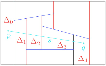
with the left end point $p$ and the right end point $q$. We want to find all trapezoids
$\Delta_0$, $\Delta_1$, $\dots,\ \Delta_k$ which the segment $s$ intersects from left to right

Figure 8.7
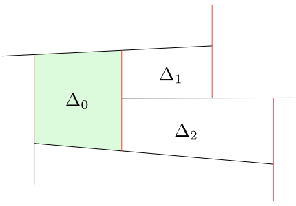
The segment $s$ passes through the trapezoids $\Delta_0, \Delta_1,\Delta_2,\Delta_3,\Delta_4$.
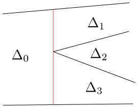
To describe this algorithm we will need the notion of adjacent trapezoids and left and right neighbours. We say that two trapezoids are adjacent if they have a common part of the vertical side that does not degenerate to a point.

Figure 8.8
Two couples of trapezoids $\Delta_0$ and $\Delta_1$, $\Delta_0$ and $\Delta_3$ are adjacent, while the couples $\Delta_0$ and $\Delta_2$ or $\Delta_1$ and $\Delta_2$ are not adjacent.
If two adjacent trapezoids have a common bottom, we say that one is the lower left or right neighbour of the other. If they have a common top, we say that one is the upper left or the right neighbour of the other.

Figure 8.9
The trapezoid $\Delta_1$ is the upper right neighbour of the trapezoid $\Delta_0$. The trapezoid $\Delta_0$ is the lower left neighbour of the trapezoid $\Delta_2$.
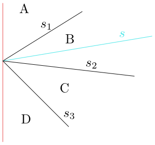
First the algorithm finds a trapezoid $\Delta_0$ in which the left end point $p$ of the segment $s$ lies. If the point $p$ is not the left end point of any segment from $S_ {i-1}$, simply use the search structure $\mathcal D(S_{i-1}) $ to find $\Delta_0$. If $p$ is the left end point of one or more segments of $S_ {i-1}$, there are more trapezoids to the right of it, and we have to select that one through which the segment $s$ runs. This is done by comparing the slopes of these segments with the slope of $s$. The slope of this segment with the end points $p$ and $q$ is equal to the quotient of the differences of $y$- and
$x$-coordinates
$$\frac{q_y-p_y}{q_x-p_x}.$$
The traced trapezoid $\Delta_0$ is characterized by the fact that its top side slope is bigger and its bottom side slope is smaller than the slope of the segment $s$.

Figure 8.10
The slope of the segment $s_1$ is bigger than the slope of $s$ and this is bigger than the slope of $s_2$. The requested trapezoid $\Delta_0$ is the trapezoid $B$.
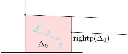
If the end point $q$ lies to the left of $\rp(\Delta_0)$, the whole segment $s$ is contained
in $\Delta_0$.

Figure 8.11
The whole segment $s$ lies in $\Delta_0$.
If the end point $q$ lies to the right of $\rp(\Delta_0)$, the segment $s$ intersects another trapezoid $\Delta_1$. This trapezoid is the lower right neighbour of $\Delta_0$, if
$\rp(\Delta_0)$ lies over $s$, and the upper right neighbour, if $\rp(\Delta_0)$ lies under
$s$. See the next picture.

Figure 8.12
Specifying $\Delta_1$ according to relative position of the segment $s$ and the point $\rp(\Delta_0)$.
In the same way we proceed further:
Algorithm FollowSegment($\mathcal T,\mathcal D,\mathcal s_i$)
Input. A trapezoidal map $\mathcal T$, a search structure $\mathcal D$ for $\mathcal T$, and a new segment $s_i$.
Output. The sequence $\Delta_0,\ldots,\Delta_k$ of trapezoids intersected by $s_i$
- Let $p$ and $q$ be the left and right endpoint of $s_i$.
- Search with $p$ in the search structure $\mathcal D$ to find $\Delta_0$.
- $j\leftarrow 0$;
- while $q$ lies to the right of $\operatorname{rightp}(\Delta_j)$
- do if $\operatorname{rightp}(\Delta_j)$ lies above $s_i$.
- then Let $\Delta_{j+1}$ be the lower right neighbor of $\Delta_j$.
- else Let $\Delta_{j+1}$ be the upper right neighbor of $\Delta_j$.
- $j\leftarrow j + 1$
- return $\Delta_0, \Delta_1,\ldots, \Delta_j$
Updating the trapezoidal map and the search structure
In this section, we show the basic idea of the algorithm that implements the 5th and 6th lines of the TrapezoidalMap algorithm, i.e. how to replace trapezoids $\Delta_0$, $\Delta_1$, $\dots, \Delta_k$ intersected by the segment $s = s_i$ by new trapezoids and so to change the trapezoidal map $\mathcal T$ and how to change related search structure $\mathcal D$.
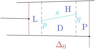
Suppose first that the whole segment $s$ lies inside one trapezoid $\Delta_0$.

Figure 8.13
The whole segment $s$ lies inside the trapezoid $\Delta_0$.
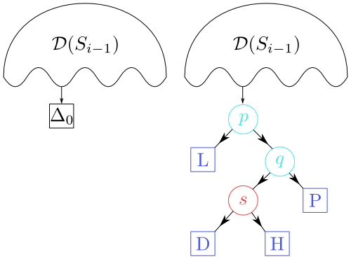
In this case the trapezoid $\Delta_0$ in $\mathcal T$ is replaced by the trapezoids $L$, $H$, $D$ a $P$. Each of them is determined by its top and bottom and by its left and right points. For example, for the trapezoid $H$ we have
$$\operatorname{top}(H)=\operatorname{top}(\Delta_0), \ \operatorname{bottom}(H)=s, \ \operatorname{leftp}(H)=p, \ \operatorname{rightp}(H)=q.$$
We carry out the modification of the related search structure in the way shown by the following figure.

Figure 8.14
The passage from $\mathcal D(S_{i-1})$ to $\mathcal D(S_i)$.
Now let the segment $s$ intersects more trapezoids.
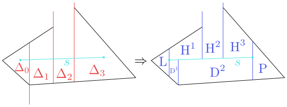
For the sake of clarity, consider the situation illustrated in the first of the two following figures.

Figure 8.15
Progress from $\mathcal T(S_{i-1})$ to $\mathcal T(S_i)$.
We replace the trapezoids $\Delta_0$, $\Delta_1$, $\Delta_2$, $\Delta_3$ by new trapezoids as follows.
$L$ is the trapezoid lying to the left of the point $p$. It has the same $\top$, $\bo$ a $\lp$ as $\Delta_0$. Since $\rp(\Delta_0)$ lies under $s$, the next trapezoid is $D^1$ with
$$\operatorname{leftp}(D^1)=p, \ \operatorname{rightp}(D^1)=\operatorname{rightp}(\Delta_0), \ \operatorname{top}(D^1)=s,\ \operatorname{bottom}(D^1)=\operatorname{bottom}(\Delta_0).$$
The right point of $\Delta_1$ lies over $s$, hence the next trapezoid lies over $s$. Denote it $H^1$. It is determined by the data
$$\operatorname{leftp}(H^1)=p, \ \operatorname{bottom}(H^1)=s, \ \operatorname{top}(H^1)=\operatorname{top}(\Delta_1), \ \operatorname{rightp}(H^1)=\operatorname{rightp}(\Delta_1).$$
The right point of $\Delta_2$ lies again over $s$, so the next new trapezoid $H^2$ will lie over $s$ and
$$\operatorname{leftp}(H^2)=\operatorname{rightp}(\Delta_1), \ \operatorname{bottom}(H^2)=s, \ \operatorname{top}(H^2)=\operatorname{top}(\Delta_2), \operatorname{rightp}(H^2)=\operatorname{rightp}(\Delta_2).$$
In the further trapezoid $\Delta_3$ there is the right end point $q$ of the segment $s$. We complete the list of new trapezoids by the trapezoid $D^2$ lying under $s$ with
the right point equal to $q$, by the trapezoid $H^3$ lying over $s$ with the right point $q$ and by the trapezoid $P$ lying to the right of $q$.
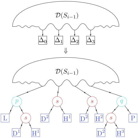
The modification of the search structure is illustrated by the following figure.

Figure 8.16
The passage from $\mathcal D(S_{i-1})$ to $\mathcal D(S_i)$.
We will not give explicit pseudocodes for updating the trapezoidal map $\mathcal T$
and the related search structure $\mathcal D$. One can create it on the basis of the previous considerations or it can be found in the bachelor thesis (in Czech)
by Ondřej Folvarčný
http://is.muni.cz/auth/th/211164/prif_b/BP.pdf?lang=cs
on pages 20 and 21.
How to remove restrictive assumptions
The simplification consisted in the fact that the different end points of the segments and
a considered point $r$ had different $x$-coordinates. We will remove this assumption by introducing shear transformation
$$\varphi(x,y)=(x+\varepsilon y,y)$$
for small $\varepsilon\gt 0$.
Lemma 8.2
For a finite set $P$ of points there is an $\varepsilon\gt 0$ such that
for any two points $p,q\in P$ holds
- $\varphi(p)_x\ne\varphi(q)_x$,
- $p_x\lt q_x\ \Rightarrow \ \varphi(p)_x\lt\varphi(q)_x$.
Proof
Let $p_x\lt q_x$. If $p_y\le q_y$, then the inequality
$ \varphi(p)_x\lt \varphi(q)_x$
holds for all $\varepsilon \gt 0$.
If $p_y\gt q_y$, then the inequality $ \varphi(p)_x\lt \varphi(q)_x$ holds if and only if
$$0\lt\varepsilon\lt \frac{q_x-p_x}{p_y-q_y}.$$
Since we choose the points $p$, $q$ from a finite fixed set, we can find sufficiently small positive $\varepsilon$ satisfying the assertion of Lemma.
If now two different points $p$ a $q$ satisfy $p_x=q_x$, it has to be $p_y\ne q_y$, and consequently also $\varphi(p)_x\ne\varphi(q)_x$.
\(\Box\)
Now, in the previous considerations, we could replace the arrangement by
$x$-coordinate with the arrangement by $x$-coordinate of $\varphi$. In fact, there is no need to compute an $\varepsilon$ to determine the transformation $\varphi$.
Lemma 8.3
For each finite set of points $P$ and a sufficiently small $\varepsilon\gt 0$, the arrangement of points $p\in P$ by $x$-coordinates of $\varphi (p)$ is the same as the lexicographic arrangement of points $p$ first according to the $x$-coordinate and then by the
$y$-coordinate.
Proof
Let $p\lt q$ in the given lexicographic order. Then either $p_x\lt q_x$ and then
according to the previous considerations $\varphi(p)_x\lt \varphi(q)_x$, or $p_x=q_x$ and $p_y\lt q_y$ and so $\varphi(p)_x\lt \varphi(q)_x$ as well.
\(\Box\)
From the previous considerations, we can make this practical conclusion: Whenever in previous considerations we find out whether a given point is to the left or to the right of another point, we will use the described lexicographic arrangement. Whenever we find out whether a point lies over or under a segment, we use the arrangement with respect to the $y$-coordinate.
Complexity estimates
Since our algorithm is random, we estimate the expected complexity both of the construction of the search structure and of the memory needed to store the search structure. Moreover, we estimate the expected running time for searching a position of a point in the trapezoidal map. Let's start with the last item.
Theorem 8.4
The expected running time for searching in the search structure $\mathcal D$ created for a random order of $n$ segments is $O(\log n)$.
Proof
The search structure $\mathcal D$ is created in $n$ steps. Consider a path for searching the position of a point $r$. Let $X_i$ be the number of nodes in this path which were added to the search structure in the $i$-th step. From figures 8.14 and 8.16 it can be seen that
$$0\le X_i\le 3.$$
Consider $X_i$ as a random variable. Then the expected time for searching is
$$E\left(\sum_{i=1}^n X_i\right)=\sum_{i=1}^n E(X_i)\le 3\text{ probability }(X_i\ne 0).$$
The fact that $X_i\ne 0$ means, that the point $r$ lies in $\mathcal T(S_i)$ in some trapezoid $\Delta$ which is constructed in the $i$-th step when adding the segment $s_i$.
At least one of the following options happens:
$$\top(\Delta)=s_i,\ \bo(\Delta)=s_i,\ \lp(\Delta)=p_i \text{ or } q_i,\ \rp(\Delta)=p_i \text{ or } q_i.$$
So the probability that $X_i\ne 0$ is at most $4/i$. The expected time for searching can be estimated from above by the sum
$$3\left(\sum_{i=1}^n \frac{4}{i}\right)=12\left(1+\sum_{i=2}^n\frac{1}{i}\right)\le
12\left(1+\int_1^n \frac{dx}{x}\right)=12(1+\log n)\\=O(\log n).$$
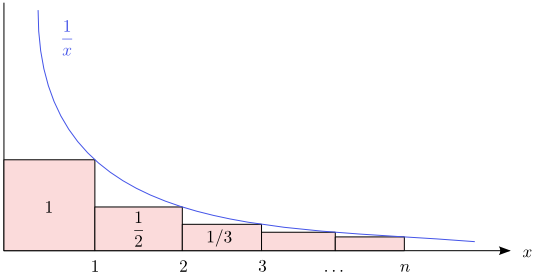
The comparison of the sum $\frac{1}{2}+\frac{1}{3}+\dots +\frac{1}{n}$
with the integral $\int_{1}^{n}\frac{dx}{x}$.

Figure 8.17
The comparison of the sum $\frac{1}{2}+\frac{1}{3}+\dots +\frac{1}{n}$ with the integral $\int_{1}^{n}\frac{dx}{x}$.
\(\Box\)
Theorem 8.5
The expected size of the search structure is $O(n)$.
Proof
The size of the search structure is
$$\text{number of leaves } + \sum_{i=1}^n \text{ number of inner nodes created in the step }i.$$
Let $u_i$ be the number of trapezoids which are constructed after adding the segment $s_i$ in the $i$-th step. In Figures 8.13, 14, 15, 16, you can see that the number of newly created internal nodes in the $i$-th step is $u_i-1$. It can be proved by induction as it is done on the page 29 of the forementioned bachelor thesis by O. Folvar\v cn\' y. Therefore, assuming $u_i$ to be a random variable, we can estimate the expected size of the data structure from above by the expression
$$O(n)+\sum_{i=1}^n E(u_i).$$
To complete the proof it suffices to prove that $E(u_i)=O(1)$.
For any trapezoid $\Delta\in \mathcal T(S_i)$ and its segment $s\in S_i$ let
\begin{equation*}
\lambda(\Delta,s) =
\begin{cases}
1, &\text{if $\Delta$ comes into being by adding the segment $s$,}\\
0, &\text{in opposite case.}
\end{cases}
\end{equation*}
Since the trapezoid $\Delta$ is determined at most by $4$ segments from $S$, we get
$$\sum_{s\in S_i}\lambda(\Delta,s)\le 4,$$
We obtain
$$\sum_{s\in S_i}\sum_{\Delta\in\mathcal T(S_i)}\lambda(\Delta,s)\le 4|\mathcal T(S_i)|\le 4(3i+1)=O(i).$$
where $|\mathcal T(S_i)|$ is the number of trapezoids in $\mathcal T(S_i)$ which we estimated by the number $3i+1$ in Theorem 8.1. Now realize that the sum
$$\sum_{\Delta\in\mathcal T(S_i)}\lambda(\Delta,s_i)$$
gives the number of trapezoids which come into being in the $i$-th step. Hence
$$E(u_i)=\frac{1}{i}\left(\sum_{s\in S_i}\Bigl(\sum_{\Delta\in\mathcal T(S_i)}\lambda(\Delta,s)\Bigr)\right)=\frac{O(i)}{i}=O(1).$$
\(\Box\)
Theorem 8.6
The algorithm constructs the search structure in expected time $O(n\log n)$.
Proof
The time for creating $\mathcal T(S_i)$ and $\mathcal D(S_i)$ from $\mathcal T(S_{i-1})$ and $\mathcal D(S_{i-1})$ is $O(u_i)$ plus a time for searching
in which trapezoid from $\mathcal T(S_{i-1})$ the left end point $p_i$ of the segment $s_i$ is lying. Its expected value can be estimated using the previous computations in this way:
$$\sum_{i=1}^n\bigl(O(E(u_i))+O(\log i)\bigr)=O(n)+O\Bigl(\sum_{i=1}^n\log i\Bigr)\le O(n)+O(n\log n)\\=O(n\log n).$$
\(\Box\)
Conclusion
The original task was to find in which face of a fixed plane subdivision a given point lies. So far we have found in which trapezoid of the trapezoidal map the point lies. Now it is easy to find a face in which the found trapezoid is contained.
It can be done if we find in which cycle of the corresponding edge-connected list the bottom of the trapezoid (taken with suitable orientation) lies.
